Canon Pixma MX340 Scanner Image Sensor Partial Reuse Ideas

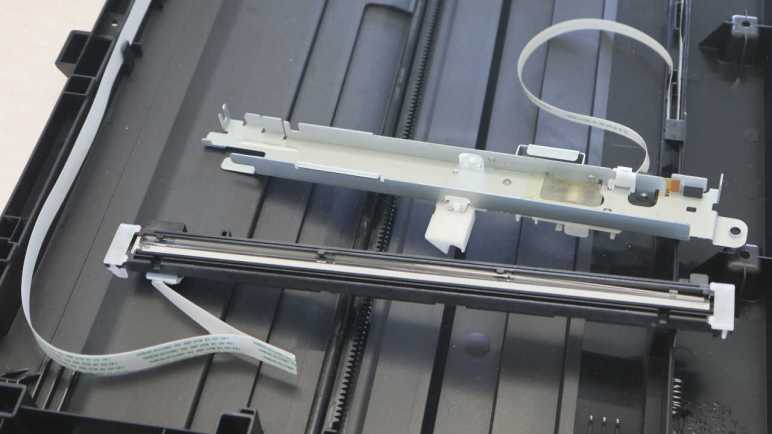
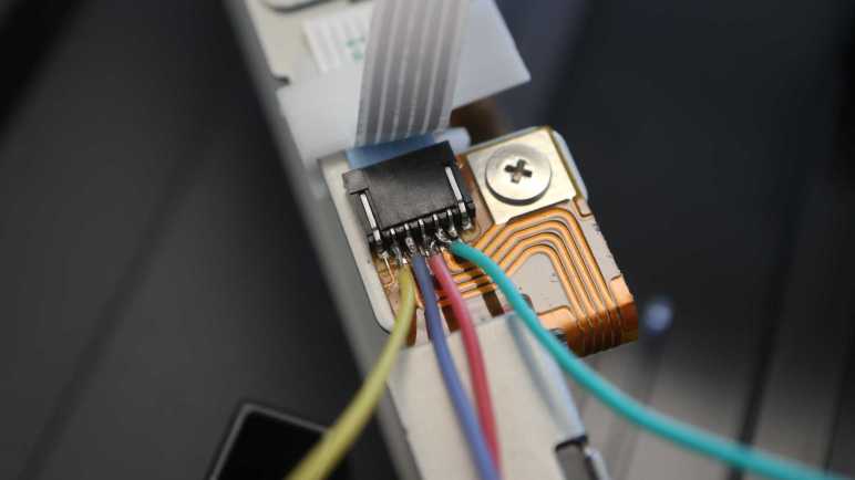
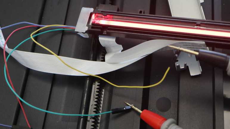
Thinking over what I now know about the scanner image sensor bar from a Canon Pixma MX340, I’ve decided using the sensor properly is beyond the reach of my current electronics projects skill level. My biggest problem is that I don’t have the tools/skills to keep up with a data clock signal running at 2.375MHz. But what if I just ignore that clock signal? For digital data, ignoring clock pulses would mean we just get gibberish. But this sensor bar communicates image data in analog voltage values. Theoretically, it is a valid option to sample that analog line at a lower rate to obtain a lower resolution image. The “new line is starting” pulse is still there at 425Hz to separate one line from the next, and keeping up with a 425Hz signal is a more tractable problem if I can get the analog sampling side figured out.

Arduino (ATmega328P)

Can an old school Arduino Nano on a ATmega328P chip keep up with the 425Hz line sync signal? I don’t know. Suppose that it could, the analog sample limit of 10k/second means (10000/425=) 23-ish samples per line or (23/8.5)=2.77 dots per inch. That’s worse resolution than a row of photo-resistors and probably not worth the effort.

ESP32

How about the ESP32 chip? It’s a much faster processor but higher core processing speed doesn’t necessarily correlate with faster ADC peripheral performance. I found this page Working with ESP32 Audio Sampling describing one effort to run the ESP32 ADC at high speed. This particular author found ESP Arduino layer to be limiting and went deeper to make some ESP-IDF calls directly.

Audio Hardware

That page got me thinking about hardware peripherals that sample an audio signal. Unlike high speed ADC chips for the industrial market, an audio-in peripheral is something available to the hobbyist market. Audio sampling usually tops out at either 44.1kHz or 48kHz, and has the advantage of being tailored for consistent performance at that sampling rate. Another advantage of the scanner image sensor pretending to be a microphone is that it’s pretty common for audio ADC to measure signal relative to a base reference ground, something I can take advantage of with the sensor pins.

The challenge of using an audio-in peripheral is splitting the incoming “audio” sample data into lines using the 425Hz line sync signal. At the moment I have no idea how I’d go about it.

I2S ADC Mode

One common protocol for communicating audio data to/from an external peripheral is I2S. Not only does ESP32 support the I2S protocol, its I2S hardware peripheral can be adapted to other high speed signal tasks unrelated to communicating audio data. At one point, Espressif offered a way to use the I2S peripheral to transfer data directly from ADC peripheral to memory at high speed. (A maximum sampling rate of 150kHz, as per old documentation for i2s_set_adc_mode.) Unfortunately, they’ve since moved i2s_adc_enable, i2s_adc_disable, and related APIs off to the “legacy” portions of ESP-IDF. The latest ESP-IDF documentation only has a short paragraph acknowledging it once existed and spoke no more of it.

Even if it was still a supported API, I saw several complaints on the ESP32 forums that the ADC is very noisy. Something I’ve found out firsthand, and apparently that limitation gets worse as we go faster. Looks like using ESP32’s onboard ADC peripheral wouldn’t be a great way to go, suggesting an external peripheral. I’ve already determined it’s not really practical to get those high-quality high-speed industrial ADCs, but maybe another microcontroller has better onboard ADC peripherals?

STM32

Searching for discussions on microcontroller ADC, I found references to chips in the very large STM32 family of products. Some have superior ADC capabilities, at least on paper. The most promising lead is ST Application Note AN5354 Getting started with the STM32H7 Series MCU 16-bit ADC. Figure 1 shows ADC behavior while sampling at 16-bit in differential mode @ 2.5 million samples per second. That’s the kind of speed needed for the scanner sensor bar!

And what’s this “differential mode”? I found a ST forum thread ADC input voltage range in differential mode where the explanation says it is a STM32 configuration using two hardware ADC channels together. The hardware will generate a single data stream from the difference between them. In other words, exactly what I want to evaluate signal+ against signal- voltage levels. Even better!

This sounds perfect. but I don’t know how the STM32H7 chips relate to the STM32F103 chips commonly available to hobbyists as the “Blue Pill” board. This is something I will need to research. I knew the “Blue Pill” is very popular with some circles of electronics hobbyists, and I’ve had requests for a STM32 Sawppy brain. If I try to do build a project around this Canon MX340 scanner sensor, it might be the motivation I need to get into STM32 development. But that’s far too big of a project for me to undertake as a side detour, so I’m going to set that aside and resume examining the electrical behavior of this inkjet. Next up: the DC motors.


This teardown ran far longer than I originally thought it would. Click here for the starting point.

Canon Pixma MX340 Scanner Image Sensor Reuse Challenges

I’ve examined the scanner image sensor from a Canon Pixma MX340 multi-function inkjet while it was still attached and running. I think I now understand how it communicates with the printer main board. However, that’s a ways from being able to reuse the sensor in my own electronics projects.

The first obstacle is that I only know voltage levels on the wires, I don’t know which component (the sensor or the main board) was responsible for putting them on the wires. Some are easy guess: the LED illumination power must come from the main board, and the image data must come from the sensor. But others are ambiguous: I see a clock signal, but who’s generating it? In order to reuse this sensor, I need to know what I need to re-implement in my own circuit in order to impersonate the printer main board.

The second obstacle is speed. My oscilloscope measured that clock signal at 2.375MHz. If my project is responsible for clock, toggling a pin in software won’t be fast enough and my current hardware skills can’t build an appropriate oscillator circuit. On the upside, if my project would be responsible for generating the clock signal, perhaps I can emit a slower clock and make everything easier. Of course, that’s out the door if clock was sensor-generated and I have to keep up. A dedicated hardware peripheral may be needed. 2.375MHz is a challenging speed for microcontroller code to keep up, demanding at least an interrupt-driven system if not other performance techniques.

Another speed-related challenge is reading and processing the analog pixel brightness value. Analog-to-digital (ADC) conversion is a common peripheral feature in many affordable microcontrollers, but they can’t sample data as fast as 2.375MHz. The basic Arduino boards built on the ATmega328P chip has a limit of 10k samples per second, two orders of magnitude too slow. That seems to be the typical ballpark for hobbyist-level hardware. Looking over Adafruit selection of ADC modules, it looks like item #5836 is the fastest unit which traded precision for speed, but that’s still only 70k samples per second.

High-speed ADC modules certainly exist, available with capabilities up to billions of samples per second. I found many listings from companies like Texas Instruments and Analog Devices. (Very appropriately named in this context.) But they’re not the kind of chips Amazon/AliExpress vendors put on breadboard-friendly breakout boards.

Given these challenges, reusing this sensor to its full potential is currently out of reach for my own projects. However, the data signal is an analog signal, and the beauty of analog systems is that we have the option of a partial (a.k.a. half-assed) implementation.


This teardown ran far longer than I originally thought it would. Click here for the starting point.

Canon Pixma MX340 Scanner Image Sensor Pinout

Taking apart a Canon Pixma MX340 multi-function inkjet, I wanted to see what I could learn from its scanner’s CIS (contact image sensor) bar. Expectations weren’t high at the start but after spending some time looking at its behavior under an oscilloscope I think I understand enough to explain every pin on its cable connector.

I’m arbitrarily numbering these pins from left-to-right in this picture. I don’t have Canon’s electronic schematic or engineering data, so this might be reversed from Canon’s actual pin ordering. I feel confident about the accuracy of red labels, I’m more tentative about the pins labeled in blue.

The first five pins support illumination. There are separate pins for red/blue/green LEDs and they all shine onto a common light guide that disperses across the sensor bar.

  1. 5.5V DC power source as common LED anode.
  2. Red LED cathode.
  3. Green LED cathode.
  4. Blue LED cathode.
  5. Chassis ground.

The remaining seven pins support image sensor data.

  1. Data clock (tentative) at 2.37538MHz with amplitude of 3.3V. Clock signals are normally square waves. This one is very nearly a smooth sine wave but I guess it still counts?
  2. Line sync+ (tentative) at 425.543Hz. Raised up to ~3.3V for one data clock cycle to signal new scan line, read on falling edge of clock signal. Low voltage level fluctuates relative to chassis ground, but is in sync with line sync- and should be compared against that.
  3. Line sync-. Reference base for pin 7 line sync+.
  4. 3.3V DC power source for image sensor logic.
  5. Power ground for image sensor logic.
  6. Analog pixel data+ (tentative). Raised up to ~3.3V above chassis ground (or roughly 2V above reference base pin analog pixel data-) to indicate brightly lit pixel. Drops to less than 0.1V above reference base for both dark pixels and overblown pixels. Drops under reference base in the non-data periods at the beginning and end of each scan line.
  7. Analog pixel data- (tentative). Reference base for pin 11 analog pixel data+. Voltage level is roughly 1.0V above chassis ground but fluctuates in sync with analog pixel+ approximately +/- 0.1V.

All of this information were inferred from using either a multimeter or an oscilloscope to observe voltage levels on each pin, while the printer is either going through its startup sequence or sitting idle. This doesn’t tell us which component is responsible for which signal. For example, while pin 11 analog pixel data is certain to come from the sensor bar, this data doesn’t tell us if the clock signal on pin 6 comes from the sensor bar or from the printer main board. That’s just the first of many barriers against repurposing this sensor bar.


This teardown ran far longer than I originally thought it would. Click here for the starting point.

Canon Pixma MX340 Contact Image Sensor Signal

I have a contact image sensor (CIS) from the scanner module of a Canon MX340 multi-function inkjet. Connecting its wires to my oscilloscope, I found a wire that I believe to convey image data.

The yellow line is probably the clock signal, and the green line fluctuates in rough correlation with sensor light levels. When the sensor bar is facing down, the signal hovers near lower voltage levels. When it is facing up towards the light, more of the signal line shows at a higher voltage. I think this is the “analog” output format for Canon contact image sensors!

If the yellow line is indeed the clock signal for each sensor pixel, and the voltage level is an analog representation of the brightness of that pixel, there is still one missing piece of data: how would we know when a scan line had completed and another begins? There must be a signal on one of the other wires, and I know there’s something that occasionally flashes past this screen. Time to chase that down.

Playing around with the oscilloscope trigger, I eventually pinned the flashing culprit down to the red wire. Its voltage is raised high for a single clock cycle at a rate of 425.543Hz. Dividing the frequency of the yellow clock signal (2.37538MHz) by 425.543 yields 5582 yellow clock cycles per red cycle. The scanner bed is 8.5 inches wide, so 5582/8.5 ~= 656. This would make sense for a 600dpi image scanner bar that is slightly wider than the scan bed.

This oscilloscope plot also shows the red signal wire voltage looks wavy, but not when compared against the blue signal wire. I think these two voltage values are intended to be evaluated together: the “new scan line” signal should be evaluated as red voltage minus blue voltage.

Keeping the oscilloscope trigger on the red wire, I changed horizontal scale to see a longer time duration. Lengthening the time scale 5000 times (from 100ns/grid to 500us/grid) showed scan lines represented by analog voltage. This particular plot shows three scan lines (one and a half scan line on either side of the trigger in the middle) and there’s a dip in the middle of each scan line. This is with the sensor bar looking up at the room ceiling so my finger is casting a shadow in the middle. I got excited that I could see some correlation between oscilloscope plot and light level, getting very close to understanding this sensor. But there’s a big problem: The shadow part looks pretty consistent, but the bright parts jump around wildly. Why is the data so noisy?

I lengthened the time scale again, by ten times to 5ms/grid so I could see about 30 scan lines at once. There’s definitely a pattern here, what is it?

Perhaps the fluctuation is normal? Since I just learned red wire voltage level appears to be relative to blue wire voltage level, maybe the image signal analog voltage is relative to another baseline. I moved the blue wire over to the pin adjacent to the signal wire to see if they fluctuate together in sync.

The good news is the baseline voltage hypothesis appears confirmed, with dark pixels dropping to the level of the newly relocated blue wire. These three scan lines show me holding my hand over the sensor bar, with several fingers casting shadows. The bad news is the non-shadowed areas are still fluctuating wildly.

I went back to staring at the earlier oscilloscope plot capture, trying to decipher a pattern to its repetition. The breakthrough came when I counted the period of repetition: at 5ms/grid, this is repeating every three grids plus a little more. So period of a little over 15ms, or a frequency somewhere under 66Hz.

Ah-Ha!

That was literally a light bulb moment: the image sensor bar is not only picking up the overhead lights, it’s picking up the 60Hz cycle of household AC power behind those lights. To test this hypothesis, I turned off my room’s overhead lights and switched to a battery-powered LED flashlight. The fluctuations disappeared, hypothesis confirmed! Now I feel pretty good about my understanding of this image sensor.


This teardown ran far longer than I originally thought it would. Click here for the starting point.

Canon Pixma MX340 Contact Image Sensor Connector

I want to see how much I can understand of the scanner image sensor bar I pulled out of a Canon MX340 multi-function inkjet. A little research side quest helped me feel better prepared for the task of figuring out what happens over the twelve wires connecting the sensor bar to the printer main board.

Looking at the copper traces on the circuit board, I can see some of them are directly wired to the pins for LED illumination. Verifying continuity between those connector pins and LED pins identified the left-most five of twelve wires. Probing for continuity with chassis ground, I found one more ground wire. Measuring the remaining wires while the system is powered up, I found one pin that held steady at 3.3V. A good power source candidate for image sensor logic.

That left five unknowns whose voltages fluctuate. Too quickly for my volt meter to catch what’s happening, hinting at data signals. My oscilloscope has four channels so I need to choose four to solder wires to and leave one for later.

This connector also has 1.0mm pitch and this time I managed to solder wires without creating bridges. Luck or improving skill I don’t know yet, either way I expect my MX340 teardown project will give me many more practice opportunities.

I turned on the MX340 and saw this on my oscilloscope screen. The yellow wire is attached to a pretty steady wave at 2.375MHz, possibly a clock signal. Its adjacent red and blue wires seem to track pretty closely to each other, the green wire looks much the same but at roughly 1V higher.

Unfortunately, that’s pretty much everything I got. I see this pattern as soon as the printer powers up, and it looks much the same during the homing sequence and afterwards. I waved my hand and shined a light at the sensor bar and saw no significant change in these signals. If I were looking at LVDS, according to Wikipedia I should see a 350mV change, but I don’t.

That said, there is something that occasionally flashes past this screen, but I didn’t know how to isolate it yet. Whatever it was, it occurred too infrequently to be image data. (Later I would determine it is a line sync signal on the red wire.)

Could the magical data wire be the fifth and final wire I had yet to examine? On paper it was a 20% chance I missed the most important wire, but Murphy’s Law raises those odds. Besides, I’m so close and it’d be silly to give up now. I turned off the printer and oscilloscope and turned on the soldering iron. The green wire was moved one pin over, and I tried again.

Jackpot! I have a candidate image sensor data signal.


This teardown ran far longer than I originally thought it would. Click here for the starting point.

Canon Contact Image Sensor

When I pulled the scanner image sensor bar from a partially disassembled Canon MX340 multi-function inkjet, I didn’t expect to understand very much of it. However, I was able to figure out the LED illumination subset of the scan head! Encouraged by this success, I felt more positive about trying to tackle the rest of the sensor bar. Which meant investing time to do a little bit of research.

When I set out to probe the electrical behavior of MX340 components, I did a brief search and found this type of sensor is called a contact image sensor (CIS). When searching for information online, getting the name is a big part of the battle. The Wikipedia page is sadly just a stub, and I don’t have the knowledge to expand it myself. (Yet?) The only source cited on that page is a ten year old link now dead, so I have to find something else.

When looking for information on electronics components at a hobbyist accessible level, I found it’s useful to search for the component and “Arduino”. Using that keyword distinguishes product sales pages from electronics details. Sadly I found nothing more helpful than the Arduino forum page that taught me the name. Searching for the name by itself found a lot of eBay listings selling replacement parts, which isn’t useful for my goal of learning about the sensors.

Scrolling through search results, my attention was caught by a link to the CIS section on Canon Components web site for businesses. This sounds like the current-day counterpart to the dead source link on Wikipedia. It is a page advertising Canon’s engineering prowess and aimed at companies that may build products around Canon CIS units. So the page exists to encourage these companies to contact the Canon sales team, which isn’t me.

Still, the page was informative. There’s a diagram breaking down the major components of Canon CIS technology, so I can get an idea of what parts I’m looking at and their names. Before seeing this diagram, I had thought the imaging sensor sits somewhere behind the clear optical lens. Now I know the clear optical lens is merely the light guide for the LED emitters I had just examined. The sensors actually look through a linear lens array adjacent to the light guide.

Armed with this knowledge, I went back to look at the sensor bar and found the row of small lenses that I had never noticed before. They are tiny, each lens is roughly 0.3mm across. As a rough approximation, that’s roughly 75 of them in an inch (~25.4mm). Scanners usually advertise their resolution as 300dpi or some multiple thereof (1200dpi, etc.) which means each of these lenses must correspond to more than one pixel in the resulting scan data. That process involves optical imaging magic out of scope of my current project: learn how they work electrically.

Clicking on the link for “Contact Image Sensor Product List” brought me to a sample selection of current Canon CIS products. I was most interested in the “Output form” column, specifying broadly how the sensor outputs its data. Possibilities include LVDS, which I have little hope of reading. Camera Link is also listed, and I had to go to Wikipedia to learn it is a protocol built on top of LVDS. And finally, there’s “analog output” which superficially seemed like the cheapest option. If I’m lucky, that’s what a cheap multi-function inkjet would have.

I don’t see any details on how image information is transmitted via Camera Link, LVDS, or analog. But I’ve learned a little more about contact image sensors today and maybe this is enough for me to recognize sensor image data when I see it under an oscilloscope.


This teardown ran far longer than I originally thought it would. Click here for the starting point.

Canon Pixma MX340 Scanner LED

I’m looking over the scanner module of a Canon Pixma MX340 multi-function inkjet. Its stepper motor got the oscilloscope treatment first, now onward to the image sensor bar.

When I took apart the scanner module, I noticed there were a few through-hole pins at the end of the image sensor bar and wondered what components they might be attached to. As I explored the scanner further to determine its startup behavior, I stared at the bar and saw the answer.

This end of the image sensor bar housed illumination light sources. This close-up shot showed the red, green, and blue LEDs working together to light the bar white.

From that I would expect three pins, one for each color, and a fourth pin as either a common anode or a common cathode. In actuality, I see five pins in this row. What did I miss? Starting with the basics, I probed the pins for continuity with chassis ground and found one, topmost in this picture.

I soldered wires to the four unknowns so I can see what they look like during printer startup, when the light bar is illuminated white looking for the homing marker.

Looks like the green wire is supplying 5.5V DC, possibly the same voltage plane powering the ADF paper sensors. The remaining three wires show a pattern that switches between two voltage levels and repeats less than 2.5 milliseconds. That works out to be less than 400Hz, too slow to be some sort of LED PWM scheme. Something else is going on. But first, I want to figure out if these wires are the positive anode (LED illuminates at higher voltage) or negative anode (LED illuminates at lower voltage).

I pulled out my LED tester and determined it is the latter: the LED illuminates from the 5.5V rail to the lower voltage shown on oscilloscope. I guess the ground pin is present merely for chassis ground and not actively used in this circuit. I also determined which wire corresponded to which colors, which is unfortunately now very confusing because I soldered these wires without knowing beforehand. Here is the mapping table:

Oscilloscope Wire ColorLED Color
YellowRed
RedGreen
BlueBlue

At least I got blue right.

Using this chart and looking back at the oscilloscope plot, I see each of the three colors are pulled low in non-overlapping time windows. The blue line (for blue LED) has the shortest time. Then the yellow line (red LED) with a slightly longer duration, and finally the red line (for green LED) for almost as long as the other two combined.

Why would the scanner light up one LED at a time and cycle through them? My hypothesis is this allows a monochrome image sensor to scan in color. Light up blue, scan. Light up red, scan again. Light up green, scan a third time. Assemble them together for full RGB color information. If so, the difference in LED illumination duration may be proportional to the image sensor’s sensitivity to those colors.

I am very happy with this discovery. It is already much further into understanding the scanner sensor bar than I had originally expected to get. Encouraged by this success, I want to see how much I can decipher of the rest of this image sensor. Which meant a quick side quest for contact image sensor research.


This teardown ran far longer than I originally thought it would. Click here for the starting point.

Canon Pixma MX340 Scanner Motor

I’m exploring the inner workings of a Canon Pixma MX340 multi-function inkjet as I take it apart. After coming up with a hypothesis on how the scanner bar finds its way to its home position, I had some fun confirming that hypothesis and confusing that electronic brain. Next I wanted to look at the motor that drives scan head movement.

Canon engineers designed the scanner bar to be easily disassembled into its two major components. A slight sideways push was all it took to separate the motor gearbox motion-control assembly from the lighting and imaging sensor bar.

Flipping the motion control assembly on its side, I can take a close look at the connector to a long cable leading back to the printer main board. There are five conductors in this wire, one of which went immediately to a screw fastening it to the stamped sheet-metal structure. This would be the chassis ground. The other four pins likely led to a pair of coils inside a stepper motor.

Probing those pins with a multi-meter, I found 15 Ohms of resistance between pairs of pins that I’ve labeled as +/- endpoints of two coils A and B.

This connector has 1mm spacing between pins (“pitch”) which is less than half of the 0.1″ (~2.54mm) pitch I’m familiar with. I’ve found this is roughly the limit of my current soldering skill, requiring two attempts before I could solder wires to them without accidental solder bridges. These wires were connected to my oscilloscope, measuring their voltage levels as the scanner went through its homing sequence.

This stepper motor is also run at 24V DC as delivered by the power supply, same as the ADF motor. The coils in this scanner motor measured 15 Ohms which calculates out to 1.6 Amps of current through each coil. Less than half of the power delivered to the ADF motor. And similar to the ADF motor, the scanner position motor does not need to hold position which means it avoids the high stress duty of having power continuously on a coil heating it up.

There’s a visibly repeating pattern in this oscilloscope snapshot, but it’s a bit difficult to make out each of the four wires when they’re all together on the same plot. Here they are individually:

Here are two ends of “A” coil, most of the time energized to one direction or another but there’s a brief period where both ends are at ground leaving the coil de-energized.

A similar pattern is visible in the B coil, offset by half a pattern period. I’m not sure why the motor cycle has this bit of de-energized coil time in between other energized patterns. Except for that small window, this pattern would be match what I expected from stepper motor operating theory. For a stepper motor spinning at a constant speed, I would expect something like this four-state cycle with equal duration per state:

A+B+
A+B-
A-B-
A-B+

But that’s not what I see in this oscilloscope trace. This is what I picked out, a slightly different pattern and some states are held for different duration.

A+B+
A+B-
A-B-
A-(off)
(off)B+

This difference from textbook description serves a purpose I couldn’t determine. Perhaps this helps ensure the coils don’t overheat from constant power? Maybe this is to help reduce resonance problems? Perhaps this is synchronized to the imaging sensor for some data purpose? It’ll stay a mystery for now, as I proceed to take a closer look at said imaging sensor.


This teardown ran far longer than I originally thought it would. Click here for the starting point.

Canon Pixma MX340 Scanner Homing Marker

I’m playing with a partially disassembled scanner module from a Canon Pixma MX340 multi-function inkjet. I’ve figured out how the scan head finds its way to its home position, and now I want to experiment with the marker used by the process. Back when I disassembled the scanner module, I had expected a mechanical homing switch but didn’t find one. I suspect the homing sequence uses a distinct pattern I found on the bottom of the bar separating the two windows.

Is this the homing marker? I will now confirm my suspicion.

The first experiment was to deliberately assemble the scanner module incorrectly. Instead of putting the lid (with glass windows) in its correct position, I placed it roughly 15cm offset in the positive direction. This was wider than the ADF window so the first test was a failure: the scan head didn’t move far enough before reversing direction. On the second test, I manually moved the scan head a bit further up, so the bar was in range of the initial positive scan. This time, the scan head homed to its new position. It also homed to the new position if I manually placed the scan head further in the positive direction: it would scan for a while, reverse direction, and find the relocated marker. Homing marker confirmed!

I then tried to see if I can spoof that marker. I measured the special pattern to start about 62mm from the document left edge. It is made of three black rectangles 20mm long and 3mm wide, separated by 20mm of white between them.

I drew up that pattern and printed it on paper. It took several attempts to actually match the measured dimensions because apparently “print at 100%” is a lie. I didn’t want to waste paper so my multiple attempts were printed on different ends and sides of the same sheet of paper.

Again I moved the scan head out of its homing position, and placed my fake homing marker paper down on the flatbed scan area. I turned on the printer and, when the scan head saw my fake marker, it acted as if it saw the real marker.

After this success, I realized that I had accidentally used one of the slightly smaller size fake markers. Retrying a few times with my different printing attempts, I found my 18mm and 19mm long markers worked just as well as the 20mm long markers. So the homing program has some tolerance for marker size.

If it is tolerant of less-than-perfect homing markers, perhaps I can spoof it with the pattern taped on a ruler? This worked when I put it on the flatbed glass like earlier experiments, but it failed if I skipped the flatbed glass and held the ruler on top of the sensor in midair. I can think of a few possible explanations:

  1. Holding the ruler above the sensor by hand had improper alignment. (It’s crooked.)
  2. Holding the ruler above the sensor by hand could not maintain the correct distance for proper image focus.
  3. The scanner sensor bar requires a sheet of glass between it and the scan subject for proper optical behavior.

And naturally, the explanation might be none of the above. I don’t feel the need to dig deeper right now because I’ve already had my fun and ready to move on to look at the motor moving this scann head.


This teardown ran far longer than I originally thought it would. Click here for the starting point.

Canon Pixma MX340 Scanner Homing Sequence

I’m carefully taking apart my old Canon Pixma MX340 multi-function inkjet, exploring its workings as I go. I’ve recorded the electrical parameters of the automatic document feeder (ADF) motor during printer startup, completing this phase of ADF exploration. My next focus is the scanner module, starting with the scan head homing sequence.

During power-up, there is a programmed sequence to ensure the scanner head is at its home position, sitting under the bar separating the small glass window (used for ADF scanning) and the large glass window for flatbed scanning. After opening up the scanner module, I could manually place the scan head at various locations to observe its homing sequence. I think I now understand how it works and writing it down here.

For the purposes of this description, I’m arbitrarily labeling the home position as zero. Movement towards the small ADF scanner window is in the negative direction, and moving down the flatbed scanner page is in the positive direction.

Usually, the scan head is already at the home position. It moves a little bit in the positive direction to verify it can detect its homing marker (more about that later) then returns to its home position.

If the scan head is not already at the home position, it will keep moving in the positive direction for a short distance. I measured this distance to be the roughly the size of the ADF scanner window. So if the scan head was located somewhere under the ADF scanner window, this motion should bring the homing marker into view.

If that short positive distance fails to detect the homing marker, the scan head reverses direction and runs for a much longer distance. I think this is the size of the large flatbed scanner window. So if the scan head was located somewhere under the large window at power-up, it will scan a bit in the wrong direction (thinking it might be under the ADF window) then course-correct back towards the zero position.

If the homing marker is not found after scanning in the negative direction for the size of the large glass, the printer enters an error state. Both its power LED and the “Alarm” LED will blink, and the LCD screen alternates between two messages: “Printer error has occurred” and “5011” which I assume is the error code indicating scan head homing failure.

It was fun to figure out how the scanner homing sequence worked, but it was even more fun to spoof that homing marker.


This teardown ran far longer than I originally thought it would. Click here for the starting point.

Canon Pixma MX340 ADF Motor

Working to understand the electronics of a Canon Pixa MX340 multi-function inkjet, I started with the automatic document feeder (ADF) on top of the machine and believe I’ve fully deciphered its paper presence sensors. Next objective is to measure the ADF motor’s electrical parameters.

Seeing four wires leading to the motor, I guessed it was a bipolar stepper motor. I disconnected its cable from the mainboard to measure resistance between each of these wires. I found two 8.8 Ohms pairs and open circuit in other combinations. This is consistent with the guess.

I didn’t find identifying labels around the perimeter. There might be something on the side facing the gearbox, but I didn’t want to disassemble it just yet.

The non-gearbox side is marked with QK1-6332 OXKT. Searching on that designation found a few eBay vendors selling replacement motors for a Canon MX340. This is oddly model-specific. I would have expected the same motor to be used across multiple devices. Perhaps this is not a designation for the motor but designation for a MX340 replacement part.

Taking advantage of the fact I still have a running printer, I soldered some wires onto the motor interface board to see their behavior during the printer’s startup sequence. The upper pair of wires (green and blue wires) is one of the 8.8-Ohm pairs, the lower pair (yellow and red) is the other pair. I expect to see four square waves alternating in a pattern consistent with driving bipolar stepper motors.

Here’s a snapshot of them during the startup sequence. Yep, bunch of square waves! I see the voltage level swings between 24V DC and ground, getting full power from the power supply. With 8.8 Ohm coils, straightforward Ohm’s Law calculation says the MX340 is driving this motor at 2.7A. Higher than I would have guessed, but within the range of power figures for a small stepper motor. It should also be noted that the ADF motor doesn’t seem to get powered on at a single coil for an extended period of time. Some stepper motor usage scenarios do this to hold position, but apparently not here. This is good because when power pulses are rapid and short in duration, the motor can tolerate higher amperage levels without burning out.

Isolating each of the wires, here’s the yellow-red coil. In the short time period of this snapshot, the coil is always energized one way or another.

And the green-blue coil doing the same. I’m not sure exactly what’s going on at the time of this particular snapshot, but it doesn’t have the regular pattern of a motor turning at a constant rate in a single direction. Perhaps I just happened to catch the motor as it switched direction? Digging for further details may be important if I am here to repair the document feeder. But as someone who only expects to repurpose the stepper motor in a future project, it is enough for me to confirm this looks reasonable for a bipolar stepper motor and knowing I can drive it at up to 2.7A at least for short periods.

That’s everything I wanted out of the ADF in this pass, I’m moving on to the scanner.


This teardown ran far longer than I originally thought it would. Click here for the starting point.