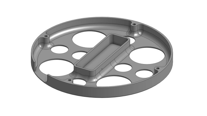
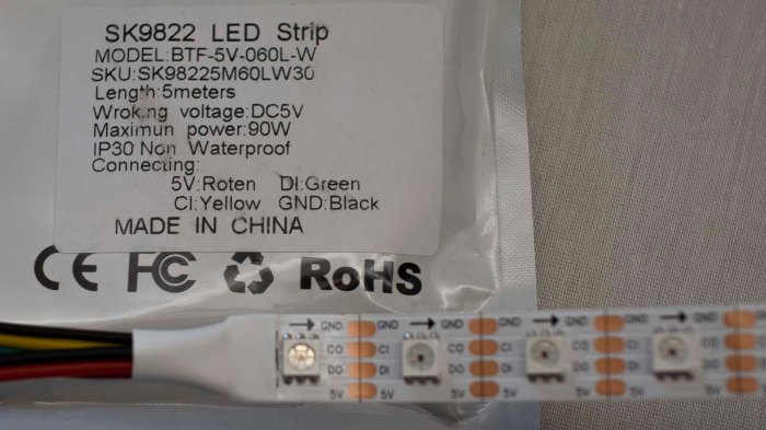
Completing first draft of a LED helix mechanical chassis means everything is in place to dig into Pixelblaze and start playing with the software end of things. There are a selection of built-in patterns on the default firmware, and they were used to verify all the electrical bits are connected correctly.

But I thought the Pixel Mapper would be the fun part, so I dove in to details on how to enter a map to represent my helical LED strip. There are two options: enter an explicit array of XYZ coordinates, or write a piece of JavaScript that generates the array programmatically. The former is useful for arrangements of LEDs that are irregularly spaced, building a shape in 3D space. But since a helix is a straightforward mathematical concept (part of why I chose it) a short bit of JavaScript should work.

There are two examples of JavaScript generating 3D maps, both represented cubes. There was a program to generate a 2D map representing a ring. My script to generate a helical map started with the “Ring” example with following modifications:

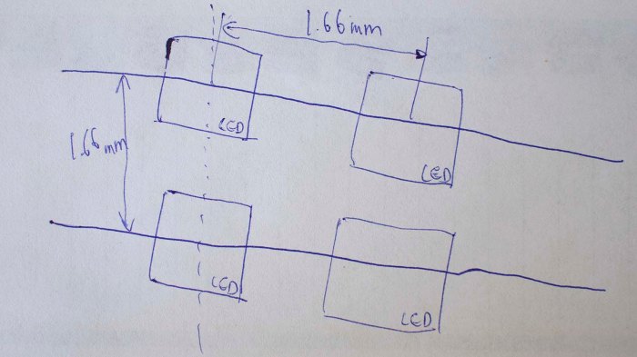
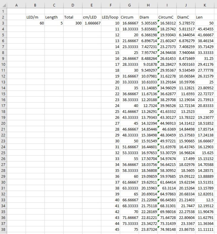
• Ring example involved a single revolution. My helix has 30 LEDs per revolution around the cylinder, making 10 loops on this 300 LED strip. So I multiplied the pixel angular step by ten.
• I’ve installed the strip starting from the top of the cylinder and winds downwards, so Z axis is decremented as we go. Hence the Z axis math is reversed from that for the cube examples.

We end with the pixel map script as follows.

function (pixelCount) {
  var map = [];
  for (i = 0; i < pixelCount; i++) {
    c = -i * 10 / pixelCount * Math.PI * 2
    map.push([Math.cos(c), Math.sin(c), 1-(i/pixelCount)])
  }
  return map
}

Tip: remember to hit “Save” before leaving the map editor! Once saved, we could run the basic render3D() pattern from Pixel Mapper documentation.

export function render3D(index, x, y) {
  hsv(x, y, z)
}

And once we see a volume in HSV color space drawn by this basic program, the next step is writing my own test program to verify coordinate axis.

I’d like my Pixelblaze LED project to be portable. A quick math session has determined while the maximum possible power draw is quite high, a battery powered design should be possible in a more realistic scenario. With that concern settled, the next decision is on choosing a physical shape for this light show.

I want a three dimensional shape because I wanted to play with a cool feature in Pixelblaze: the Pixel Mapper. This feature allows me to specify a mapping from pixel order to their physical location. Then I can write my LED pattern in terms of physical position either in 2D (x,y) or 3D (x,y,z) coordinates, and let the Pixel Mapper figure out how individual LEDs will correspond to my pattern. This allows me to decouple a pattern’s logical behavior from a specific rig’s physical layout, allowing fun tricks like creating a pattern works equally well on 300 or 10,000 LEDs, just by changing over to a new mapping in Pixel Mapper. This would be an extremely powerful creative tool if I could get it to work for me!

Backing off from big dreams, I return to my 5 meter spool of 300 LEDs on a single strip. To support projects like mine, these strips were designed to be cut apart and rearranged. Solder pads are exposed so we could electrically connect them back into a single chain, no matter their physical arrangement. This sent me into analysis paralysis for a while trying to decide how to cut them up and how to rearrange them. Eventually I decided to do the easiest thing: I’ll use the strip in a single segment, no cuts.

The most basic way to create a 3D geometry from a single line is to curve it into a helix. In addition to not requiring any cuts or resoldering work, it also avoids sharp bends which these strips have only a limited tolerance for. A cylindrical shape is an easy introduction into the 3D space of pixel mapping, a “Hello World” before I tackle future projects with more sophisticated geometry.

Next step: designing a chassis for my helical LED strip.

Once our Pixelblaze is configured for a local WiFi network and type of LED strip, the next step is to actually make that electrical connection. It is also time to unplug the Pixelblaze from our computer, because once our LED strip is connected we will need more power than what a computer USB port can safely deliver.

For this particular project, my Pixelblaze will be controlling one of these (*) built from SK9822 LED modules, they are signal compatible with APA102 which is one of the control data types supported by Pixelblaze. This strip is 5 meters long with 60 LED modules per meter for a total of 300 pixels. That’s more LEDs than what I can track in my head, but well within a Pixelblaze’s ability as it could drive thousands of LEDs.

This particular package had a label which described the role of each wire. Not all of them have this information presented, and we have to determine 5V and GND rails using a meter. But even when we have a convenient label this time around, it is still worthwhile to double check. Not every LED strip vendor follows wiring convention: the red wire is not always 5V and the black wire is not always GND. Getting it wrong could destroy both our LED strip and our Pixelblaze. [UPDATE: Good news! Pixelblaze V3 features reverse polarity protection so it would gracefully tolerate reversed +5V / GND without damage, until we realize our mistake and rewire it correctly.]

Thankfully these strips were designed to be cut to length, with solderable pads for each of the four lines. This means we have conveniently accessible pads to check for continuity between a GND pad and (what we believe to be) GND wire, and 5V pad to 5V wire.

Thankfully it is less critical to get data and clock lines right. A mixup would mean nonsensical patterns or no patterns at all, but no permanent damage. For this particular strip, the data and clock lines were inverted from the order on Pixelblaze circuit board hence the yellow/green crossover visible in this picture.

The row of headers visible on the right is an expansion bus, capable of hosting the optional sensor expansion board which I plan to incorporate into this project down the line.

Because I had configured my strip settings to be at low (10%) brightness, I could power this entire rig with a portable USB power bank advertised to deliver up to 2A. This was enough to verify I could run prebuilt patterns on my newly connected LED strip. But how much more power might this setup draw? Time to do some math and figure it out.

(*) Disclosure: As an Amazon Associate I earn from qualifying purchases.

A Pixelblaze is a small board who generates data signals for a color LED strip to display interesting dynamic patterns. These patterns are described via a program written in a web-based editor running on the Pixelblaze itself. It is a nifty little self-contained unit for projects that involve a large number of individually addressable LEDs. I have a prototype Pixelblaze V3 on hand for a candidate project. I’ll be using my blog here to publish a first draft of Pixelblaze general setup and configuration information, as well as documenting my work to apply a Pixelblaze to a specific LED project.

The first thing to do with a freshly unpacked Pixelblaze is to connect it directly to a computer’s USB port. A standard computer USB port will not provide enough power to drive a large LED strip, but it is a stable and known power source. It is useful for verifying a Pixelblaze was undamaged in shipping and for performing initial setup.

Less than a minute after being plugged in, a new Pixelblaze would show itself as an open WiFi access point our device could connect to.

Once connected, open a web browser and try to load any URL, we will be redirected to Pixelblaze WiFi Settings menu. The browser will complain there’s no internet access but this is expected: we’re just using this to connect to an actual WiFi access point. Select the network we want to use and login.

Optional: check the discovery service box. Because after this step is complete, Pixelblaze will not longer be an open access point: it would have joined the new network. To reconnect to Pixelblaze and resume setup, we will need to know its IP address. If this is not possible (or just inconvenient) check the discovery service box. This is an optional feature to let a Pixelblaze announce its address on a network.

Once Pixelblaze’s own WiFi access point disappears, our device can rejoin the original network and visit http://discover.electromage.com to see addresses for discovery-enabled Pixelblaze on the same network.

If discovery is not enabled and the Pixelblaze IP address is known, we can point our web browser to that address. Or if discovery is enabled, we can clicking “Open” from the Pixelblaze Discovery Service list. Once a Pixelblaze is configured for a WiFi network, the “Saved Patterns” menu is where it will start.

Change to Strip Settings menu to configure our Pixelblaze for our LED strip.

Name: This will show a Pixelblaze default name, we can optionally replace it with a friendlier one.

Brightness: This is a slider bar that defaults to 100% brightness. In the case of most LED strips, this will be a blindingly bright setting that consumes a lot of power. For our initial test and experimentation, we don’t need to blind ourselves or burn that much power. Move that slider lower: somewhere in the 10-20% range will still be easily visible.

LED Type: Change this to match the communication protocol used by the LED strip that the Pixelblaze will be driving. If the modules on a LED strip is not on the list, check online to see which of the listed modules are compatible and select that. Example: SK9822 LEDs are compatible with APA102, so we can select APA102 for LED strips that use SK9822 modules.

Pixels: Change this to match the number of modules on the LED display that the Pixelblaze will be driving. Example: a 5 meter long strip with 60 LEDs per meter will have a total of 5 * 60 = 300 pixels.

Data Speed: Leave this setting alone for now.

Color Order: Leave this setting alone for now.

Once the Strip Settings have been updated to match our intended LED output device, we shift our focus to hardware. Unplug the Pixelblaze from our computer, and warm up our soldering iron, it’s time to connect LED strip to Pixelblaze.